Regularization and tricks for shape generation

Introduction

This post is the continuation of my project on generating artworks with neural nets. The first post was here

The objective is to be able to easily draw what the computer produce. But the objective ends up to be : how to force the computer to produce something that will have less friction to produce when using pens and paper.

Using color in optimization

What are the challenges ?

Color is a continuous spectrum. However, we have only a limited number of pens and thus available colors.

We need a way to get back to this set of colors.

Thus we have two options :

• predefine the available colors at start
  • you can use the precise colors available
  • but you need to know in advance which colors will be used by the network
• quantize the colors after the optimization
  • free optimization with a postprocessing step
  • but we might have something very different from the original depending on the quantization
  • quantization cannot be learned in the diffvg framework

Implementation of the post optimization quantization

I have already explored some ideas on how color quantization could be applied in previous posts : 1, 2.

However, here, we can go for something rather simple : fitting a Kmeans on the Lab color space of all the curve produced.

Lab color space is more adapted for our color perception and will provide more satisfying visual results.

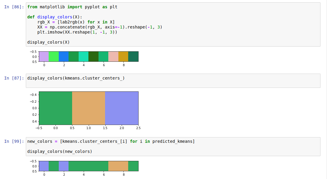
How the quantization is done with Lab and Kmeans. The visualization of the clusters colors and the quantization process looks reasonable.

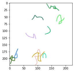
Here, we take a set of svg curves and apply the quantization defined before. The process looks smooth.

Recombining with previous optimizations

The quantization usually looks good, but we don’t know how much we have damaged the original image from the point of view of the neural net.

One idea is to re-optimize the image given, this time, the fixed set of colors.

Here we see green and black lines that move a little bit.

We also use the multi-scale recombination from previous post to get a bigger image for a lower optimization cost

Here is an example

• The initial learned pattern

• and the final image obtained with finetuned quantization :

Adding regularization in the optimization

What are the challenges ?

To give a bit of context on the optimization process, this page can give you the main formulas.

In short, we have two main elements that will dictate what will appear in the image :

• which network do we use
• which channel of a given layer will be maximised

Once, this has been chosen. The optimization will try to fill as much space with the pattern that maximize the layer activation. This leads to having a very dense final image.

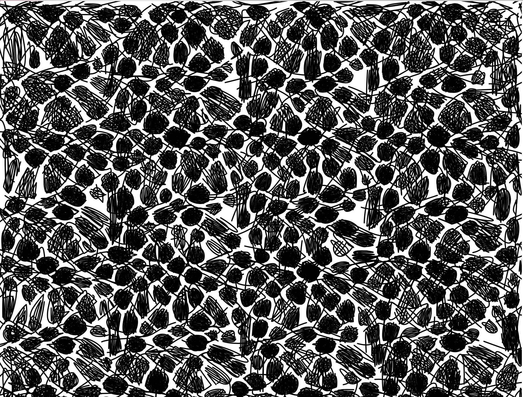
The patterns are very interesting. But from the human point of view, it can be a bit overwhelming.

If we are interested in forcing sparsity, how could be incorporate this constraint in the loss ?

A parallel with neural style transfer

Neural style has known a lot of fame when the tech was new. One could mix a pony picture with its favorite painting!

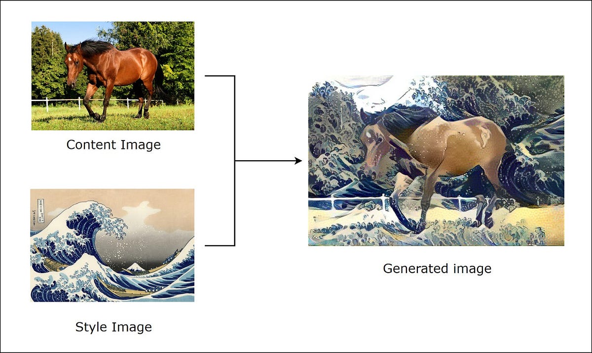
We are interested in the format of the loss. We usually minimize the following terms :

• A content loss given by a gram matrix difference between the learned image and the content image (the horse)
• A style loss given by a gram matrix difference between the learned image and the style image (the painting)

In this setting, we identify our problem as :

• The content loss is given by optimizing for a given layer in our neural net
• The style loss could be taken in the same format as in neural style transfer and become a regularization

In terms of equation, we would have something like :

loss = content_loss + style_regularization + other_regularisation
loss = -sum( VGG_16(optimized_img, content_layer) ) + lambda * norm( Gram(VGG_16(optimized_img, style_layer)) - Gram(VGG_16(style_img, style_layer)) )

For the sake of simplicity, we use VGG_16 as both the content and style network.

However, the style and content layer might probably be different. Conv2_2 might be the style one and Conv4_3 might be the content one. We also need to introduce a style image that will dictate its properties through the style loss.

Practical results

Let’s get practical ! In order to get a sparsity regularization, we use the following Mondrian painting. The large amount of white space allow (we hope) to create the desired sparsity.

We omitted a detail in the previous section, we need to find a lambda to balance the content loss with the style regularization. Experimentation showed that a value of 50 seemed to balance both terms. But this parameter seems to have a lot of effect in some cases and very little on other.

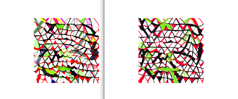
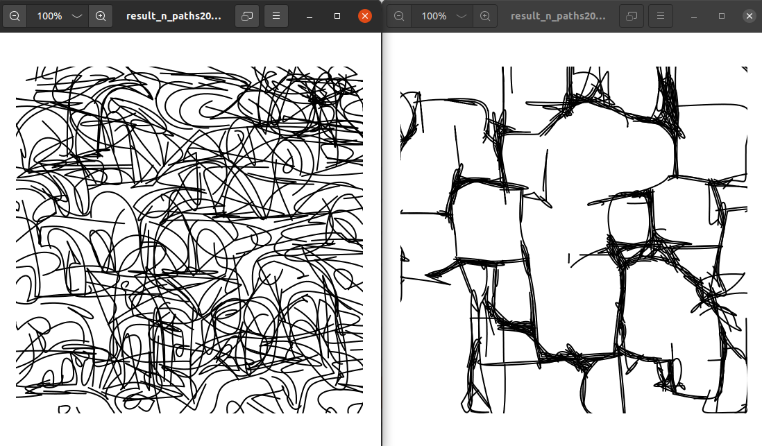
In the following pictures, we show :

• on the left, the unconstrained optimization process
• on the right, the one with the new style regularization

One of the best example of regularization taking place.

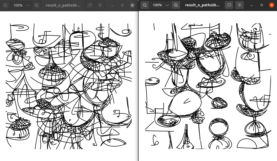
When the feature is not adapted, we can see that the generation collapses to a primitive Mondrian.

In some case, the effect can also be limited. We still observe some benefits

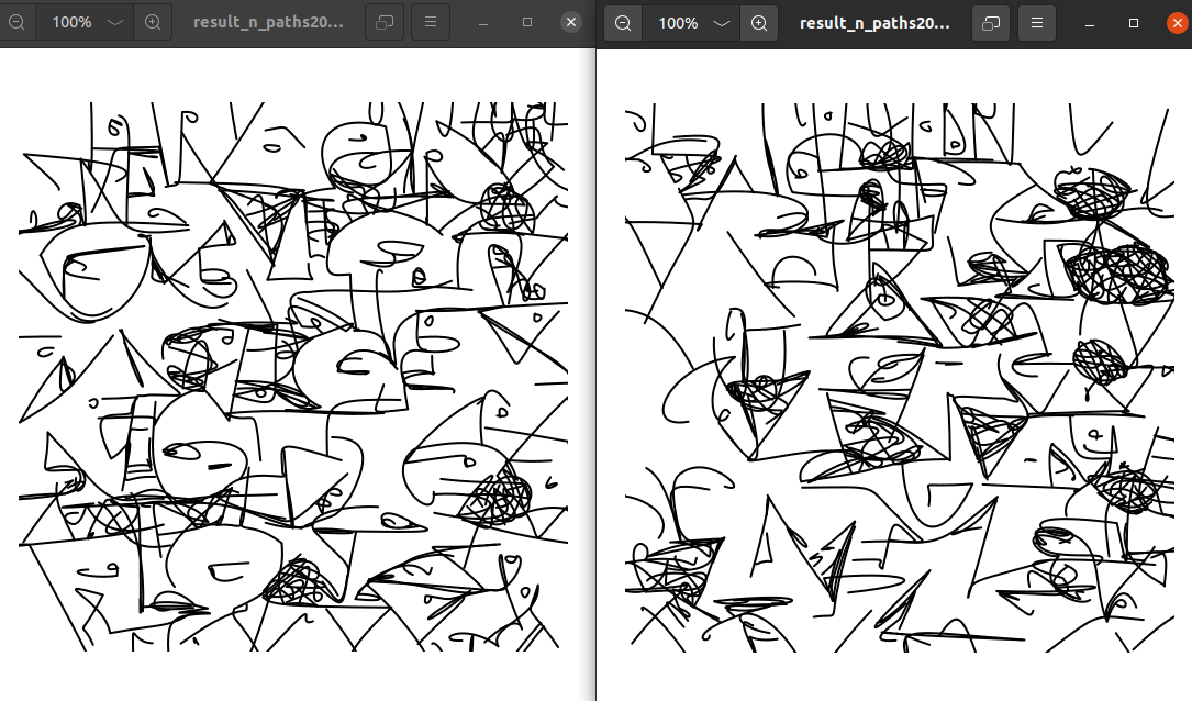
An example with the usage of color, a stronger regularization is needed to have a visible result.

From left to right, regularization=0, 50, 1000. Results at 50 are barely noticable.

Case study

We look for a specific case where things work out and try to observe what the improvment is. Even though it looks like cherry-picking, we believe we might learn from this new process how to better optimize in the future.

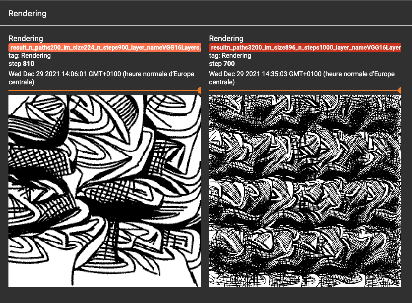
In order to spot good cases, we use Tensorboard to log all experiments with and without the regularization. Then channel index, we identify interesting cases.

We spot the following screenshot by this approach :

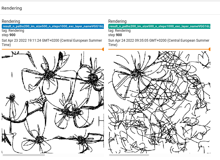
Interestingly, we have more patterns in the version with regularization (on the left).

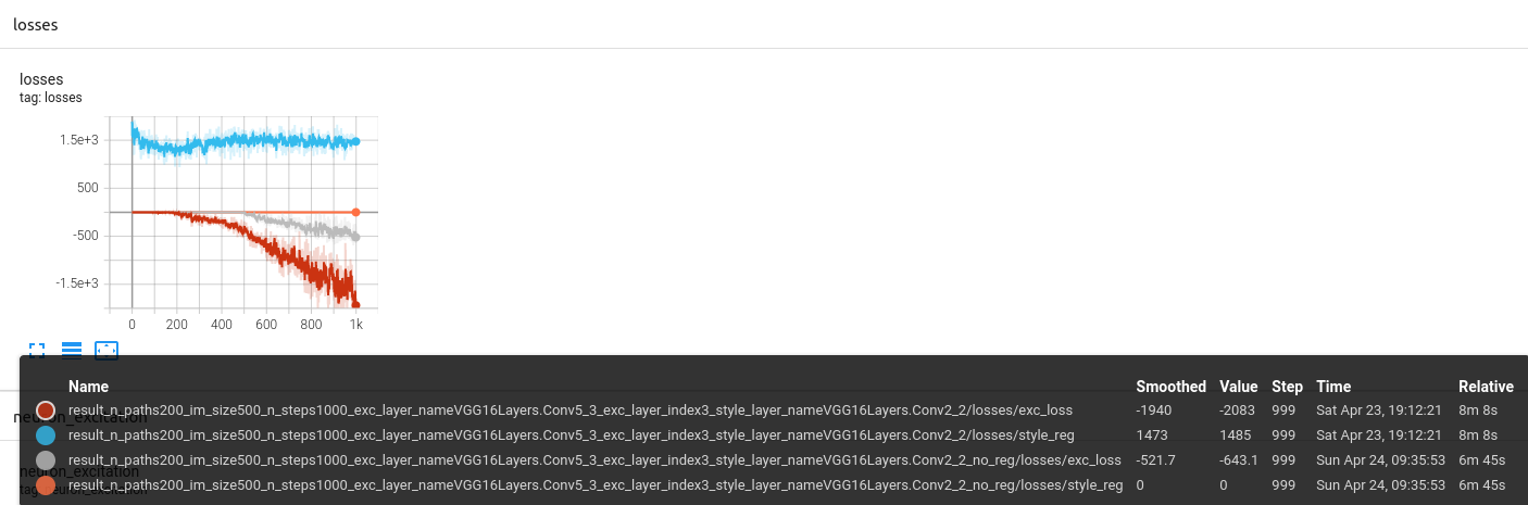
A much more surprising observation is that the loss with regularization converges to a better point than the one without.

to read this graph :

• look at the no_reg ending, we observe a style_reg value of 0 in this case
• for the optimization with regularization, we observe a much lower exc_loss corresponding to the main objective of the optimization

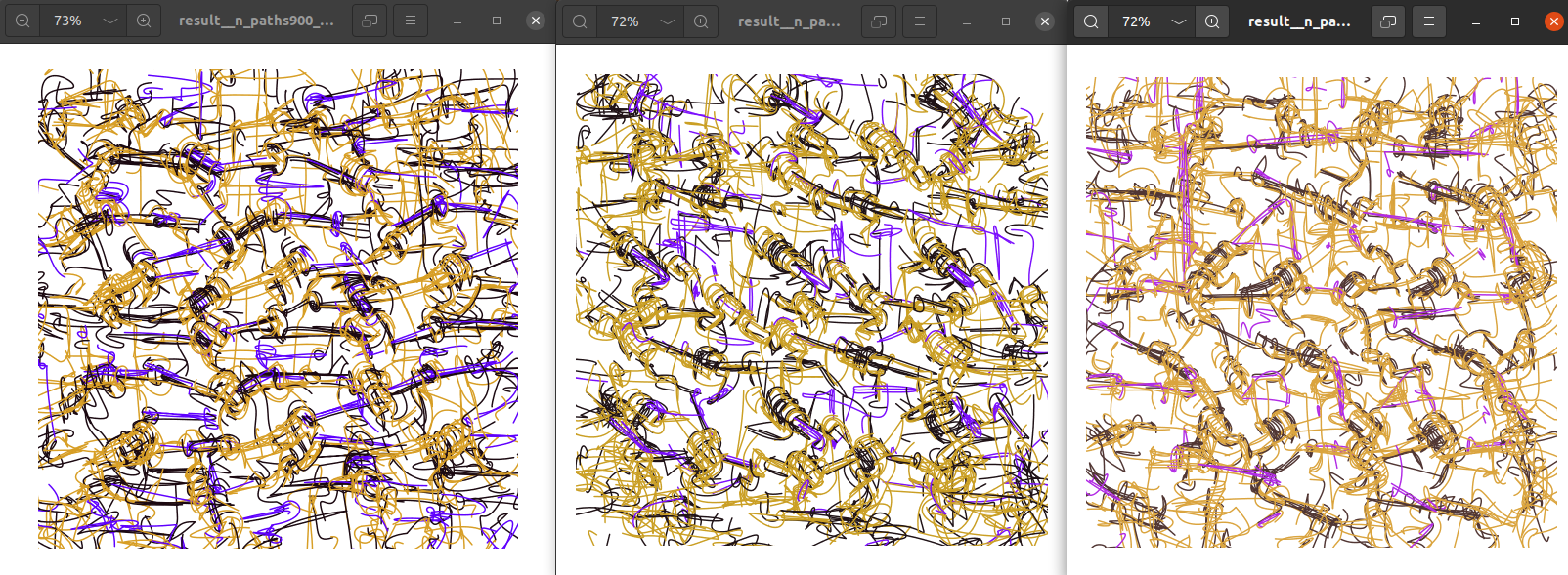
Is this an isolated case ?

Here are two other example, that suggest the opposite.

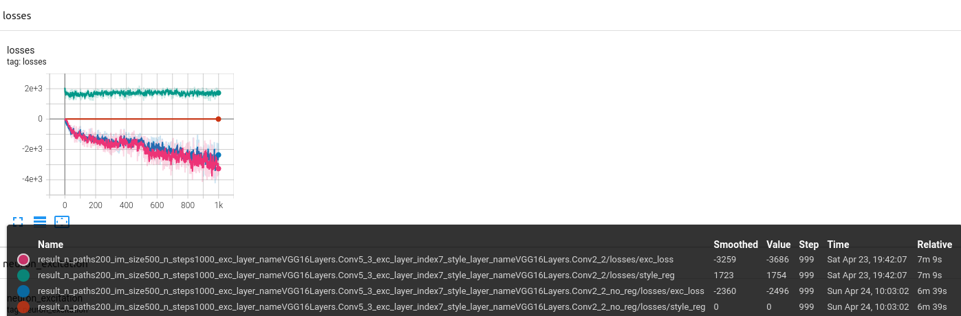
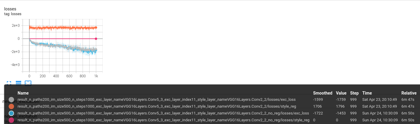
It looks like it isn’t as other examples were found in the multiple generations. But this property is not granted for every run, it is probably partially a side effect of the style image chosen.

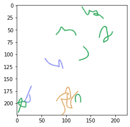
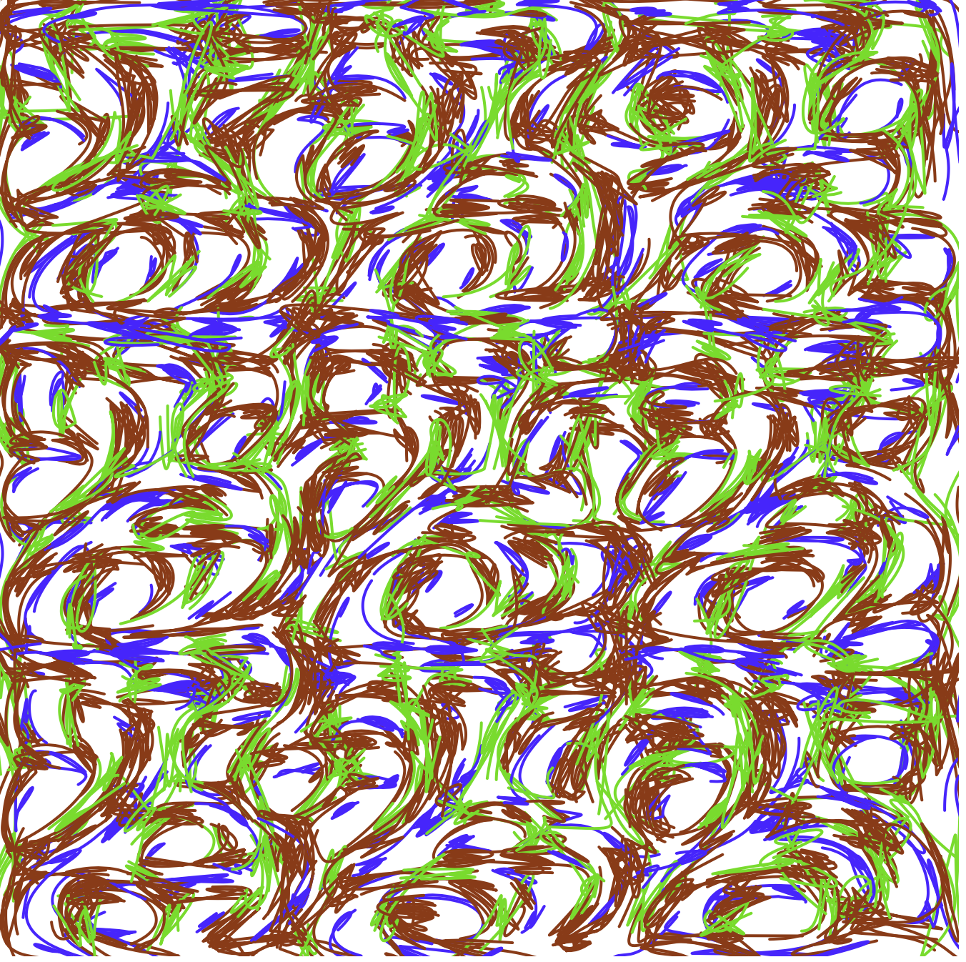
Some generations

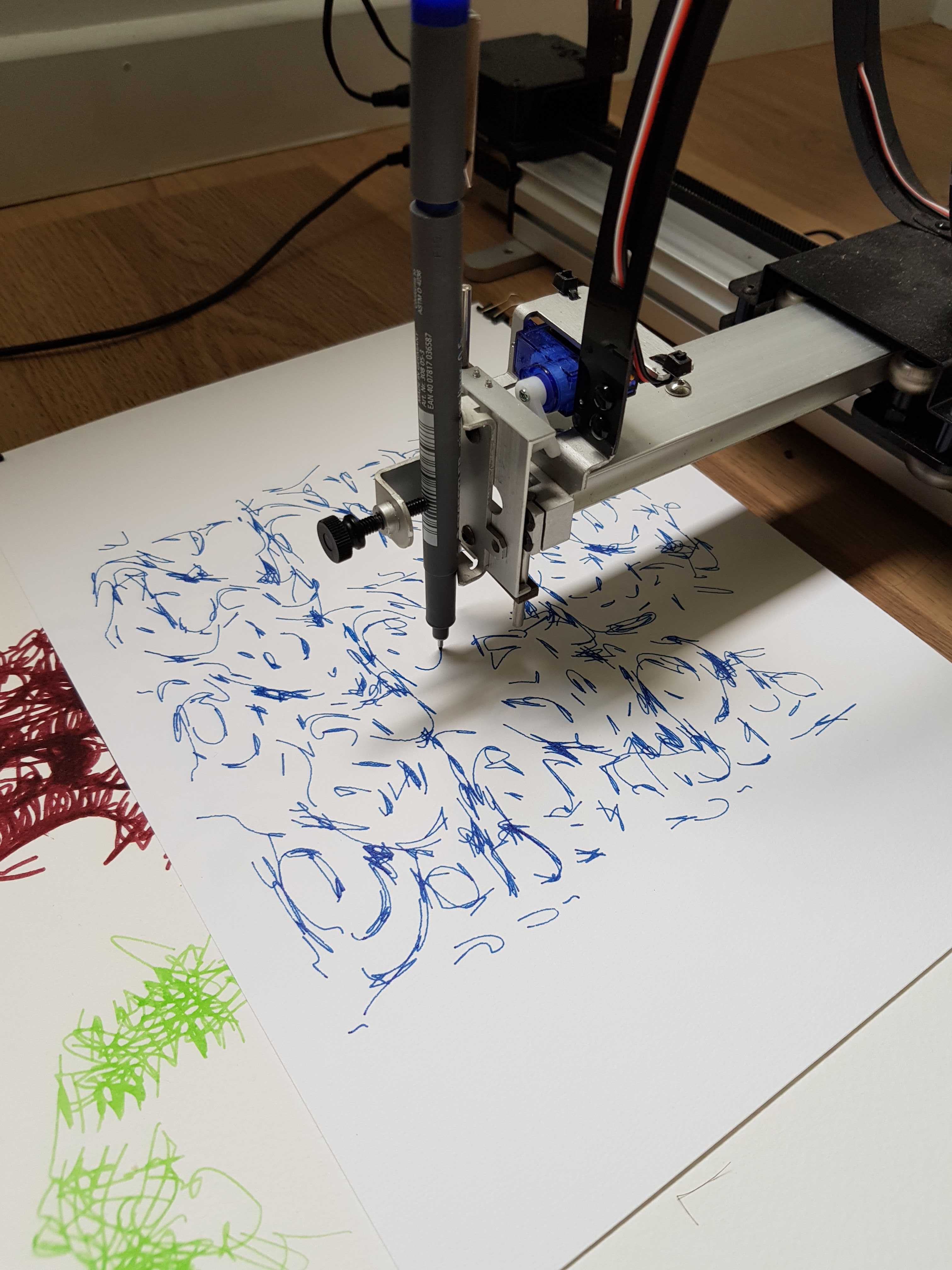
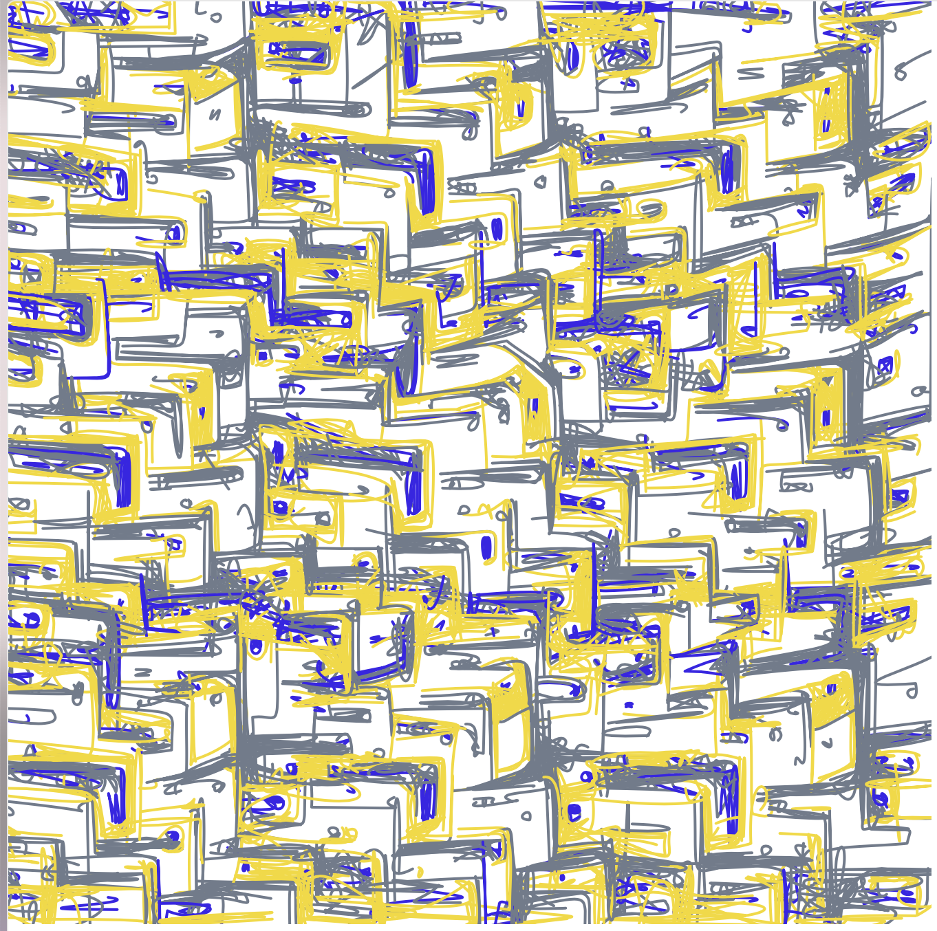
One example of colored optimization in svg format.

The result once printed.

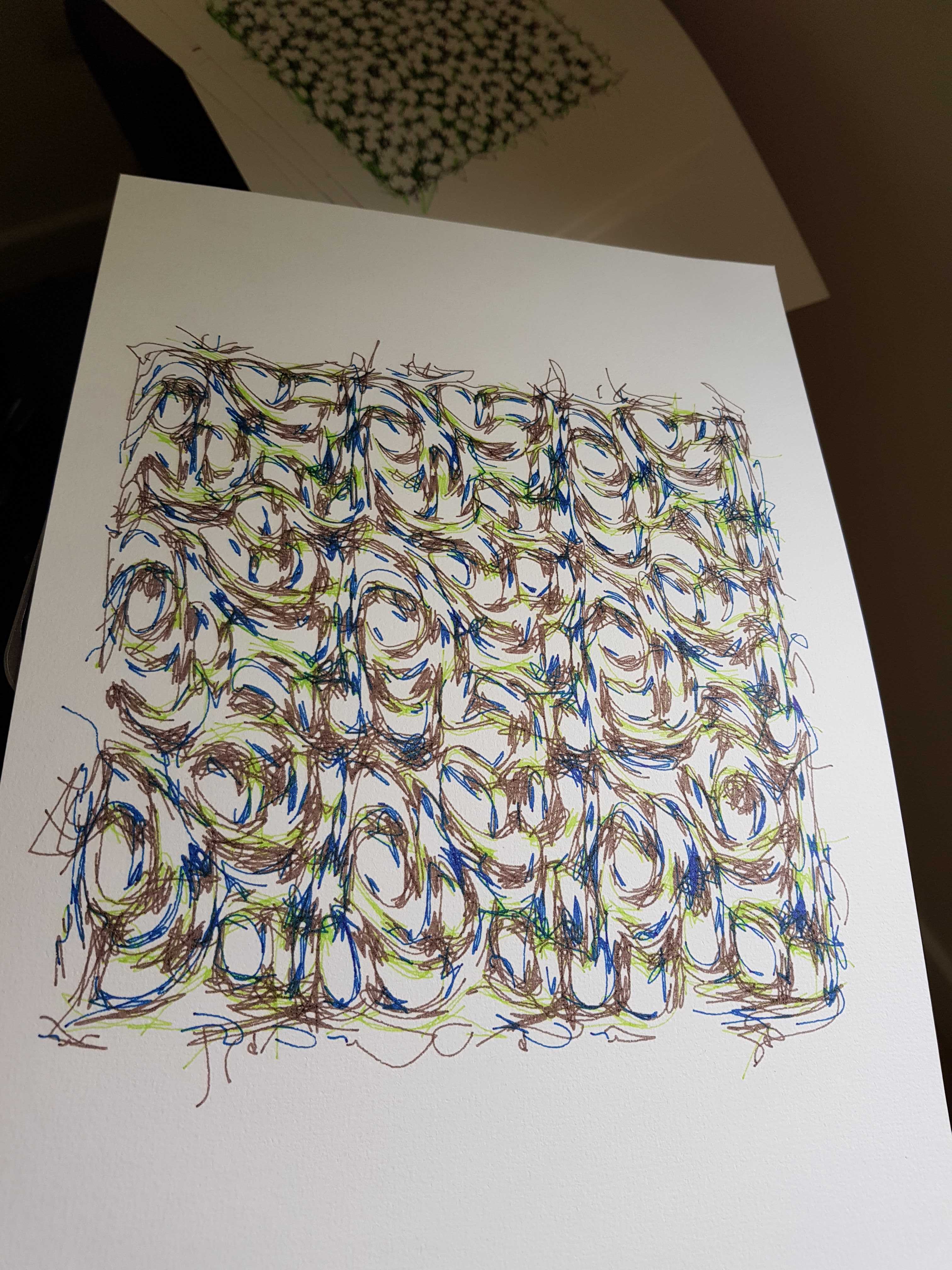
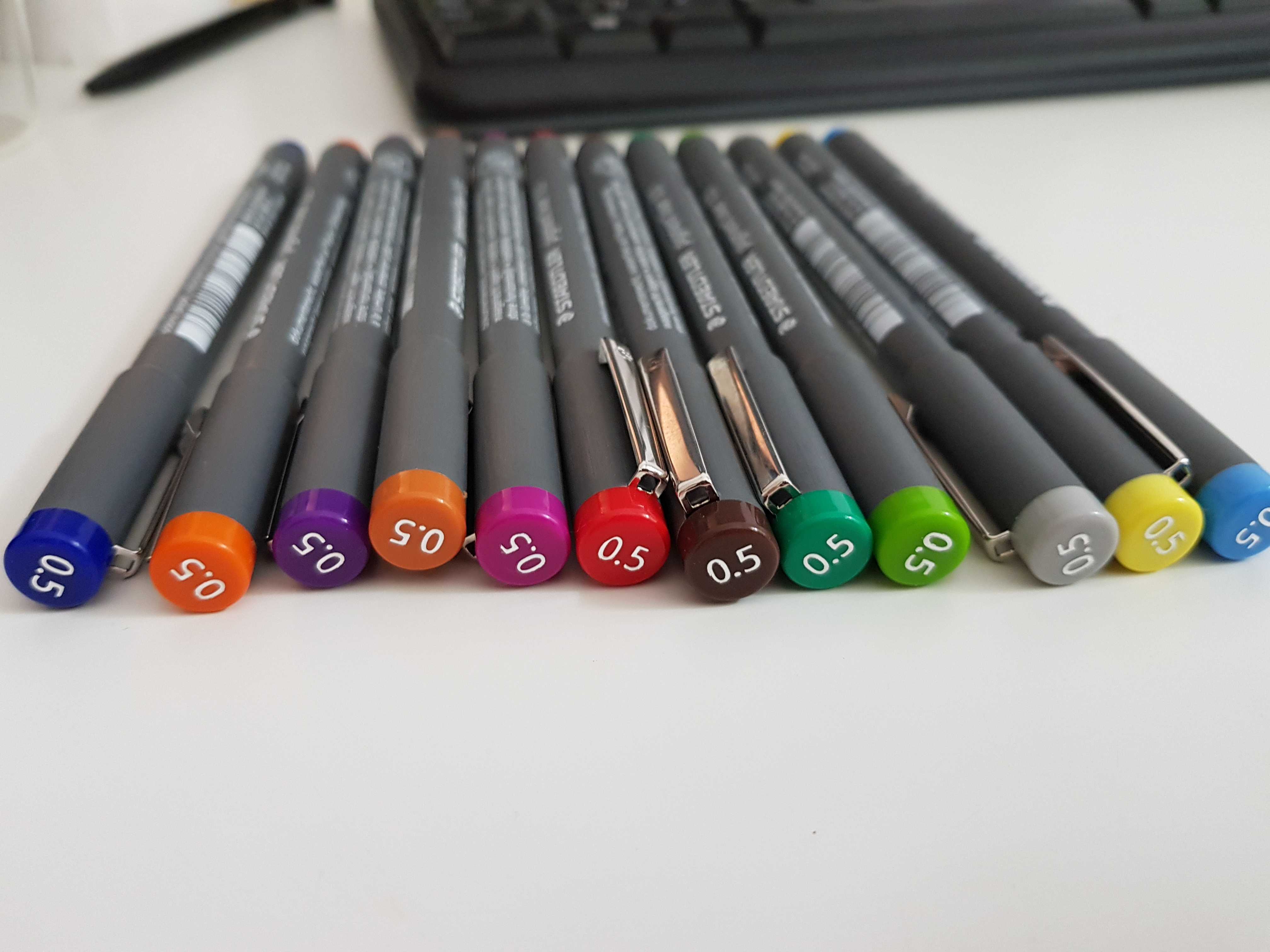
We do not have a 1-to-1 match because of svg layers that cannot be easily reproduced with plotting. The colors are also difficult to reproduce. A bright blue is very complicated to execute with pen ink.