Plotting densely filled images

Introduction

In the previous post, we have seen ideas to handle plottable colors in neuron excitation.

However, we remained at a very basic level of transformation. The quantization process can be very rough and does not respect the transparency that was used in the original optimization process.

In this blog post, we will dive deeper on methods for truthful post hoc color quantization process.

In short :

1 - We improve the basic algorithm for quantization and observe the qualitative results

2 - Using an alternative generation process, we improve the previous method with transparency handling

TLDR

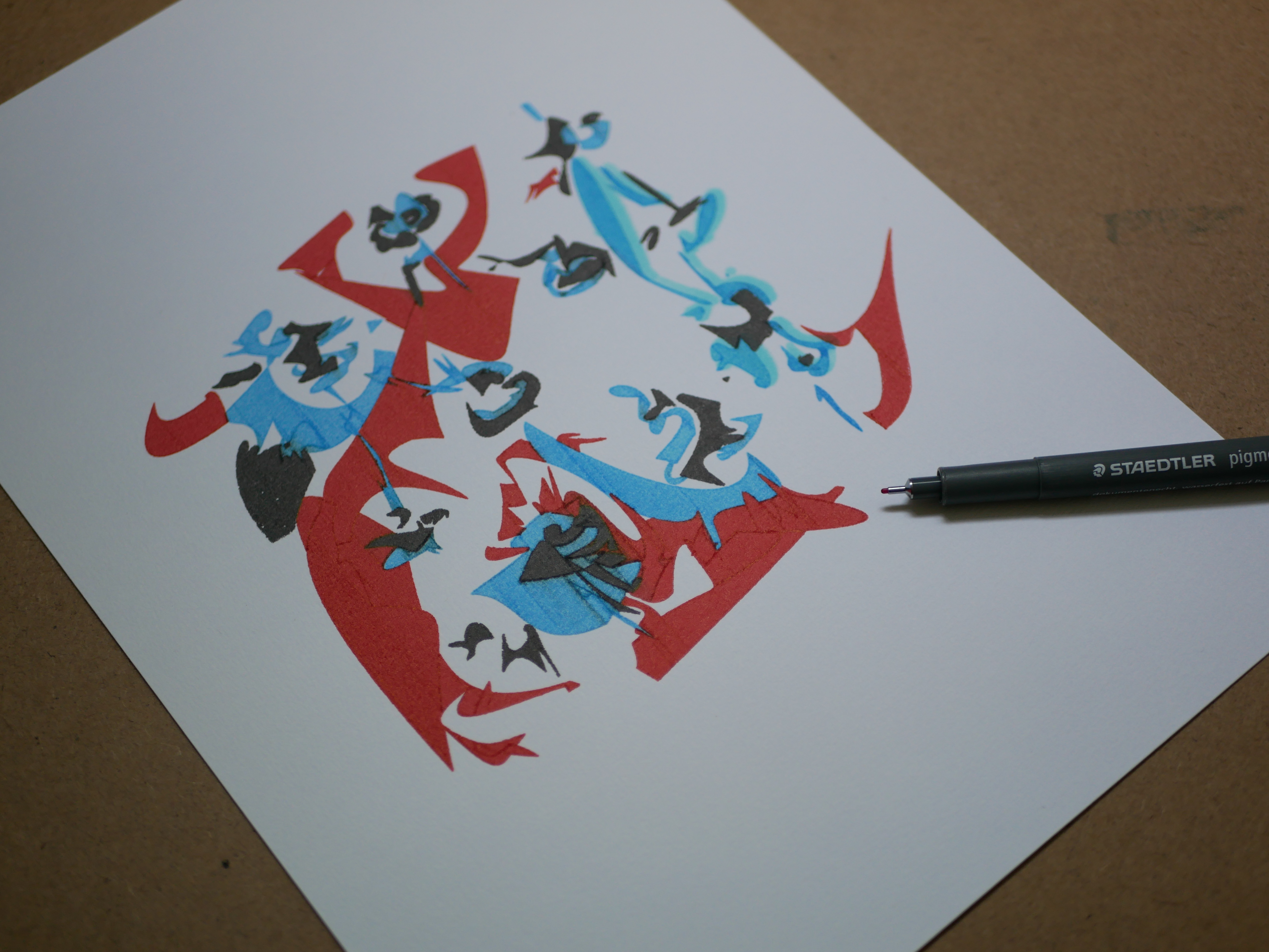
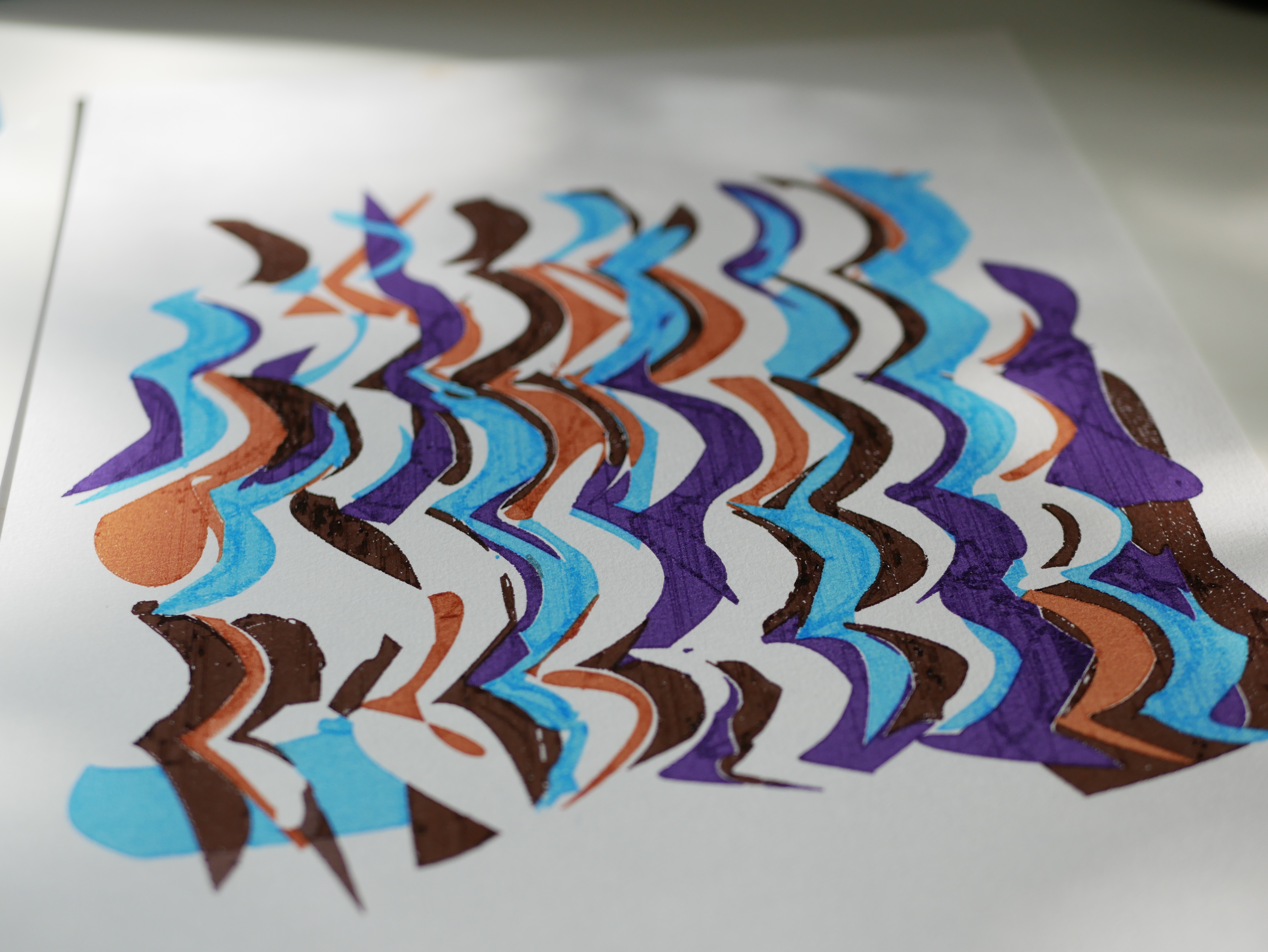
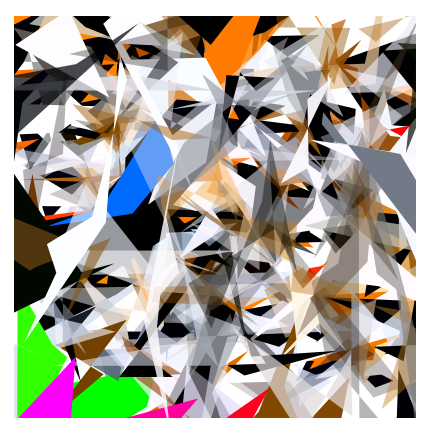
We get this kind of production

Stroke based images and their shortcomings

Review of the plots from the previous posts

Optimization using free form curves gives initially interesting pictures. But during the postprocessing that allows to make it plottable, we lose the magic touch that makes it interesting.

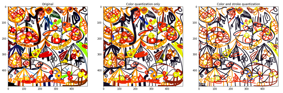
In this example, we quantize the number of color and stroke width.

What’s next ?

Given the unsatisfactory results on the previous color quantization methodology, we want to rethink our approach.

We avoided two main elements in the previous approach :

• curves are more than points, they are in fact polygons
• the color quantization should take into account the mixing of color between curves

The problem remains hard with this new setup :

• computing multiple intersections and covers is hard
• the curves are 3rd order bezier, making their intersection non-regular polygons

Despite the difficulty, we pursue this direction as the main improvement possibility.

Using polygons as optimization basis

From the previous section, we understood that we need to be able to compute the precise intersection of shapes in order to assign the right quantized color.

One possible solution is to change the optimization basis from curves to polygon. And this is totally doable with Diffvg.

From there, we need to rework the svg generation process to use this different basis.

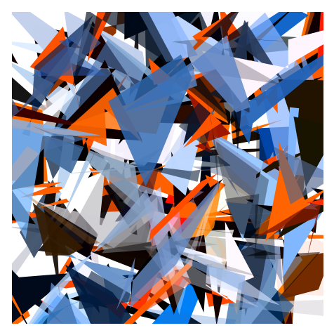
The two captions display result of optimization based on polygons.

Reducing the number of used polygons with LIVE

LIVE is an improvement over diffvg for painterly rendering.

Using a few tricks, the same image can be produced using far less polygons :

• Incremental addition of new shapes along a partial optimization process
• Shape positions are not initialised at random rather depending on where the reconstruction error is maximum
• A new constraint on curves to avoid self interaction

This will help a lot as the intersection problem is at least O(n2)

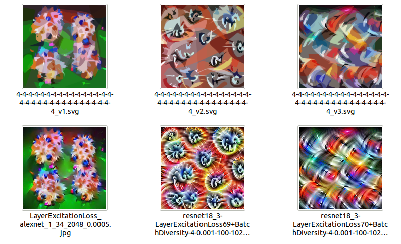
These three captions display the reconstruction result from jpg images. We observe a major simplification but the final images only has 128 shapes.

Color quantization

Once we have a limited number of shape, we can decide which color we will use.

# Outlook of the algorithm
Input :  We have N polygon with different colors and stroke size
Output : We have the same set of polygon but with colors limited to a given collection C_n

After this light introduction, let’s look at the precise algorithm.

K-means

The different colors used on the shapes are 4 dimensional : 3 RGB channel plus an alpha one.

The alpha one is important in our problem as it allows to have several shapes on the same spot contributing to a color mix.

The final algorithm is as follows :

# Get color from each curve, in Lab format and alpha removed
X = [rgb2lab(c.color[:3] * c.color[:3]) for c in curves] 
# Stroke width weighting allows to have larger stroke color better represented
W = [c.stroke_width for c in curves]
kmeans = KMeans(n_clusters=n_quantized_colors)
kmeans.fit(X, sample_weights=W)
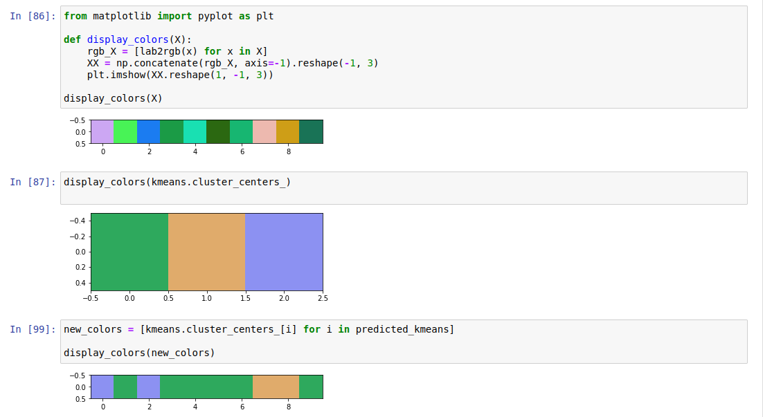
display_colors(kmeans._centers)

This gives a simplification as illustrated in this image

Ransac

RANSAC is a technic commonly used to remove outliers.

Why do we need it ?

Because a few curves shapes to have colors completely off the limited palette we would like to have.

K-means may not be resistant to this kind of data as its centers may shift in the direction of the outlier or even occupy a center if enough colours are allowed. However outlier removal should be used carefully as sparsely used color can sometimes be fundamental in the rendering of the image.

In this picture, we can see chunks of blue that do not contribute to the harmony of the picture. We would like to remove them from the final palette.

What is the pseudo code for our ransac ?

k = ... #n umber of sampled colors
X, W = ... # curve colors and curve strokes used as weighting
N = X.shape[0] # The number of curves
for i in ransac_tries:
    n_sampled_this_round = randint(0.5 * N, N)
    index_sampled = random.choice(range(N), n_sampled_this_round, replacement=False, p=W)
    X_sampled, W_sampled = X[index_sampled], W[index_sampled]
    kmeans = Kmeans(n_clusters=k).fit(X_sampled, sample_weight=W_sampled)
    score = kmeans.score(X_sampled, W_sampled) / sum(W_sampled)
    results.append((kmeans, score))
return sorted(results, key=lambda x: x[1], ascending=False)[0]

The main steps :

• Sample n out of N curves based on the weights as density
• Fit a new kmeans with this n elements
• Compute the average score (= agreement among the sampled points on the quantized colors)
• Finally keep the kmeans that has the best score

Below, we can see the difference between the

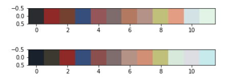
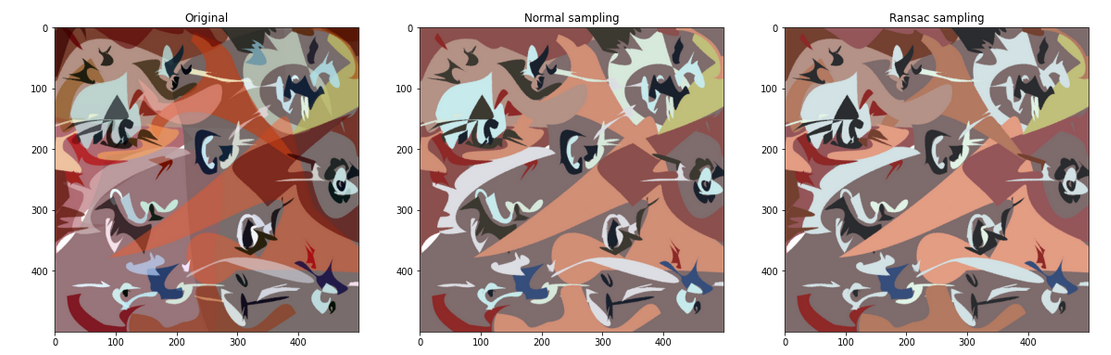
We often get cases where a color is replaced by another and it improves the final results.

Computing regions covers

So far, we have seen how color quantization can be done given our set of shapes.

But we did not handle very seriously the transparency.

Pixel cover

One way to handle transparency is to use the pixelated rendering of svg.

The uniform grid sampling guarantees that the collected colors will be representative of the final rendering.

From the previous code snippet, we need to change only two things :

X = rendered_image.reshape(-1, 3)
W = None

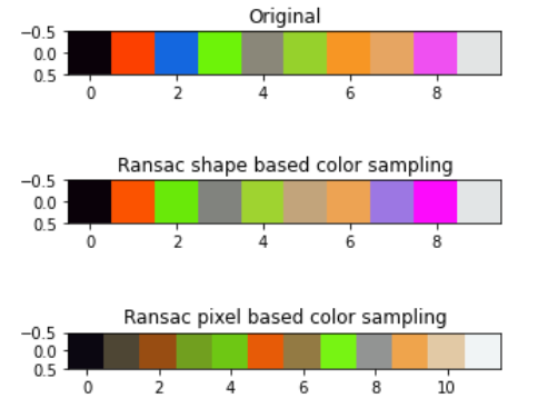
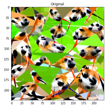
The change is simple and produce meaningful color when looking at the original image.

So why didn’t we do it IN THE FIRST PLACE ?

Because it cannot be simply applied to our shapes. We need to backtrack what pixel values mean at the shape level.

Luckily, this is what we will do in the next section.

Shape cover

So far we used polygons to represent the shapes in the image. However, this is not enough when we want to plot it with pen.

When viewing an image, layering is taken into account, plotter tools don’t take this into account, this must be computed manually.

In short, we need to carve away for each layer the space occupied by the layer above.

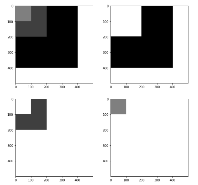
In this example, we have 3 full square of different color in the first image. The 3 subsequent images show how we should transform the squares to be able to plot the image.

From this basic idea, we compute the final image as :

• a set of intersections of all shapes
• the difference of all shapes from these polygons

Algorithm

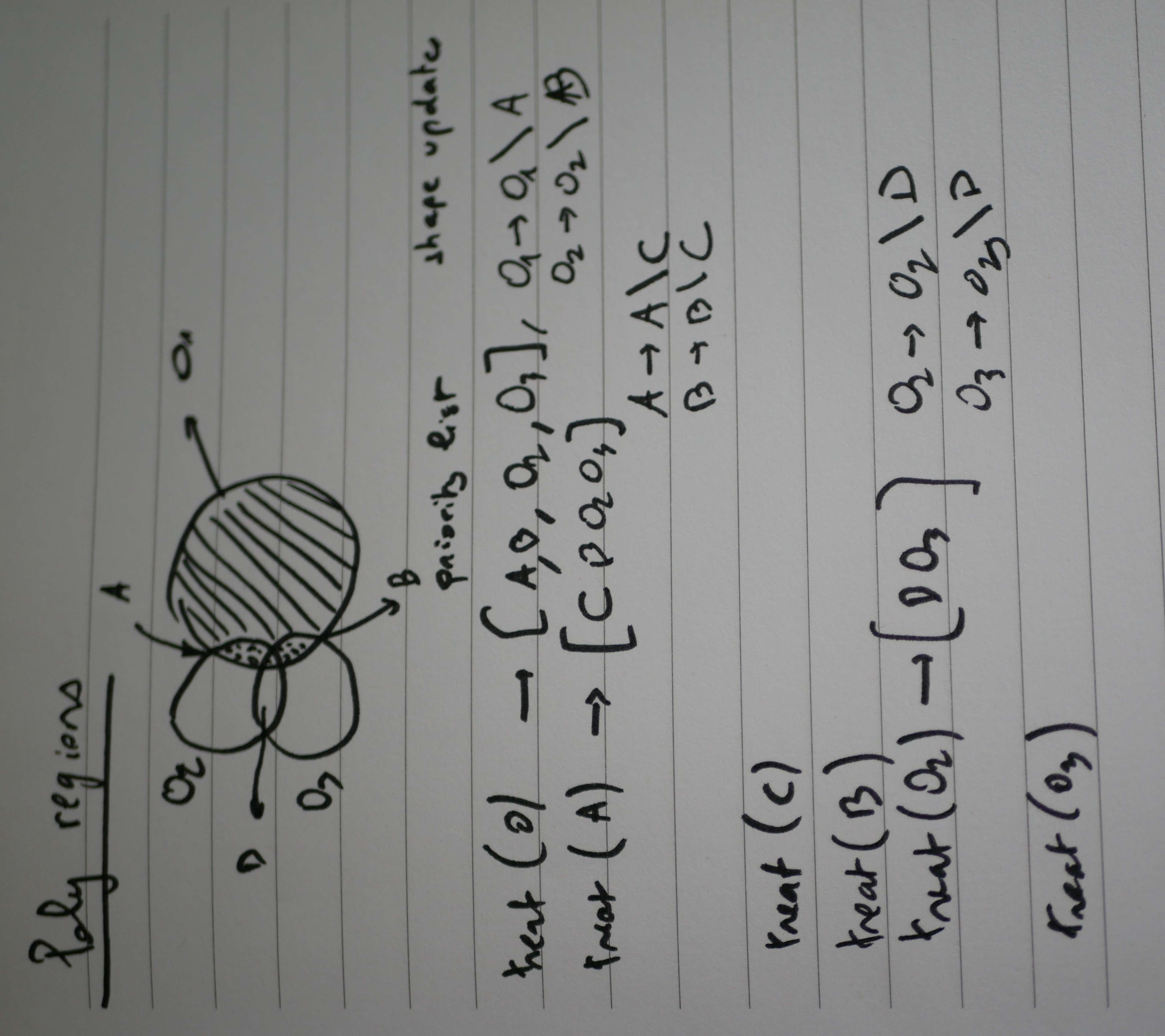
Details :

• We start with 3 shapes O1, O2, O3 : O1 being the higher up
• treat function compute the required intersections
• first line depicts what happens when the function is run on 01
  • We get two intersections A and B
  • A and B must be removed from O1, O2 and O3 as they will hold different colors
  • A and B are pushed on top of the priority list
• next, A is treated
  • its intersection with B, named C, is an intersection with 3 shapes
  • Again C is removed from B and pushed to the priority list
  • No more intersection exist between C and another polygon, regular operation will resume
• B, D, O2 and O3 are regular or similar cases

Plotting time and conclusion

You have already seen the results of this technic at the start of the article.

However, some challenge around the simplification of the shape remain to be solved :

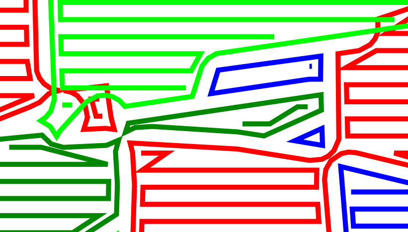
• 1 - Over fragmentation

This picture display the lines the plotter follows in order to produce the physical rendering.

We can see how multiple regions are incorrectly not fused into a single layer of color. All the small fragments will be visible in the final rendering and this will be detrimental to the look of the artwork.

• 2 - Processing time : with around 5 to 10 minutes to compute the cover, there is probably a huge area of improvement.

• 3 - Scale and pen size adaptation : pen strokes of different colour should not intersect, another small round of post-processing is necessary

This picture displays the trajectory of the plotter again. When wanting to join isolated segments, we might end creating bridges between separated layers.

This should be avoided at all cost.

In conclusion, we have an interesting new direction in order to plot more complex drawings. But the complexity cost of this new technic is relatively high and will need additional adjustments in order to produce clean results 100% of the time.