Feature visualisation : more!
How to regularize the generated image
In the previous article, we have seen how to generate img that maximize an intermediate layer of a neural network.
If you remember the optimization formula, you noticed the total variation term \(TV(I) = \Sigma_i ||I(i+1) - I(i)||^2\). This term is relatively empirical, we know it will reduce high frequencies by construction, but we don’t control its effects on the image. Moreover the filter was designed for grayscale and doesn’t take into account the differences between the different colour channels.
I’m going to quickly review what was presented in this two articles https://distill.pub/2017/feature-visualization/ https://distill.pub/2018/differentiable-parameterizations/ and explain how we can improve our regularization.
Image transformations as regularization
One way to have a stable image that maximize a feature layer is to force the image to have almost invariant activation across few pixel translation and few degree rotation.
To be able to do that, we need an original image that will be optimized and a set of transformations. With PyTorch, we can build a tensor that is the concatenation of the original image transformed with a random factor. We then optimized this tensor instead of the image alone. If the transformation is differentiable, the original image will be modified. Exactly like when training a neural net for classification, we can use the data augmentation trick to better learn an image representation.
 The same principle can be use to train robustly a neural net or an image
Let’s have a look at how we can do the translation in PyTorch :
def jitter(tau, img):
    B, C, H, W = img.shape
    tau_x = random.randint(tau, 2 * tau)
    tau_y = random.randint(tau, 2 * tau)
    padded = torch.nn.ReflectionPad2d(tau + 1)(img)
    return padded[:, :, tau_x:tau_x + H, tau_y: tau_y + W]
We use the original image, pad it and crop the same size with a small bias tau in x or y directions. In fact, the intermediate tensor is built that can later backpropagate to the individual pixels of the base image.
The code for the rotation and small scaling follows the same idea.
def scaled_rotation(x, in_theta=None, scale=None):

    if in_theta is None:
        in_theta = random.choice(list(range(-8, 9)))
    rad_theta = math.pi / 360 * in_theta

    if scale is None:
        scale = random.choice([0.95, 0.975, 1, 1.025, 1.05])

    if x.shape == 4:
        B = x.shape[0]
    else:
        B = 1

    theta = torch.zeros((B, 2, 3))
    theta[0, 0, 0] = math.cos(rad_theta)
    theta[0, 0, 1] = -math.sin(rad_theta)
    theta[0, 1, 0] = math.sin(rad_theta)
    theta[0, 1, 1] = math.cos(rad_theta)

    grid = scale * F.affine_grid(theta, x.shape)
    return F.grid_sample(x, grid)
The useful tool here is the grid_sample function that allows subsampling with float factors and keeps differiability propagation.
class Rotation(nn.Module):
    def __init__(self, in_theta=None, scale=None):
        super().__init__()
        B = 4
        theta = torch.zeros((B, 2, 3))
        for i in range(B):
            if in_theta is None:
                in_theta = random.choice(list(range(-8, 9)))
            rad_theta = math.pi / 360 * in_theta
            if scale is None:
                scale = random.choice([0.95, 0.975, 1, 1.025, 1.05])
            theta[i, 0, 0] = math.cos(rad_theta)
            theta[i, 0, 1] = -math.sin(rad_theta)
            theta[i, 1, 0] = math.sin(rad_theta)
            theta[i, 1, 1] = math.cos(rad_theta)
        self.grid = nn.Parameter(scale * F.affine_grid(theta, [B, 3, 224, 224]))
    def forward(self, x):
        y = torch.cat([x for _ in range(4)], dim=0)
        z = F.grid_sample(y, self.grid)
        return z

r = Rotation()
with SummaryWriter(log_dir="./logs") as w:
     w.add_graph(r, x)
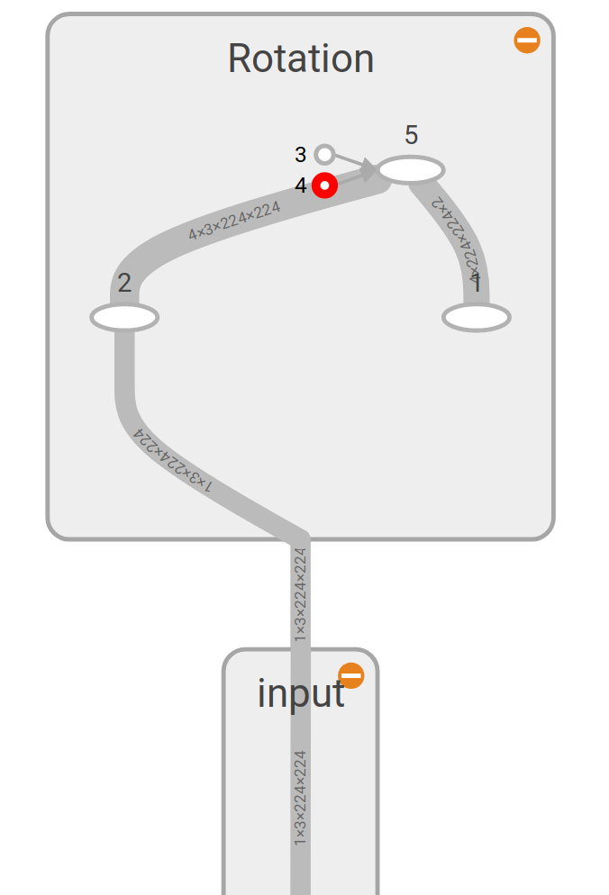
This gives us the following series of operations. Our input image is given by the index 0, it is replicated in 4 on operation 2 and 4 different rotations and scale are applied on operation 5.
Original image preconditioning
Transformations are not the only way to regularize our image, we can also change the space from which it is optimized. Fourier space makes sense as a single change in the frequency domain impacts the whole image.
What is suggested in the Distill article and present in the Lucid Library is to optimize a complex Fourier image rather than the raw RGB space image. On top of that, the color channel should not just be RGB but taken from a decorrelated space (aka coming from a PCA like transformation). The decorrelated space to RGB is learned through PCA from ImageNet data, let’s have a look at how we can do this.
$XX^T = PDP^{-1}$
import torchvision
import numpy as np

d = torchvision.datasets.CIFAR10("./", download=True)
dd = d.train_data - np.mean(np.mean(np.mean(d.train_data, axis=0), axis=0), axis=0)
B, H, W, C = dd.shape

x = dd.reshape(-1, 3)
xx = x.transpose().dot(x) / (B * H * W)

d = decomposition.PCA(3)
d.fit(xx)

print(d.components_)
We found the matrix P that defines the mapping from our uncorrelated space to the RGB space found in CIFAR10. $X_{real} = P * X_{uncorrelated}$ with $X_{uncorrelated} = FFT^{-1}(X_{optimized})$
Now, we can have a look at the image transformation from the Fourier space. With the following code, we are going to build the image in the Fourier space and transform it back into normal rgb.
def build_freq_img(h, w, ch=3, b=2, sd=None, torch_var=True):
    freqs = _rfft2d_freqs(h, w)
    fh, fw = freqs.shape
    sd = sd or 0.1
    init_val = sd * np.random.randn(b, 2, ch, fh, fw).astype("float32")

    if torch_var:
        spectrum_var = torch.autograd.Variable(torch.tensor(init_val, requires_grad=True))
    else:
        spectrum_var = torch.tensor(init_val)

    return spectrum_var

def freq_to_rgb(spectrum_var, h, w, ch=3, decay_power=1, decorrelate=True):
    spectrum_var = normalise(spectrum_var, h, w, decay_power)
    img = torch.irfft(spectrum_var, 3)
    rgb_img = img[:, :ch, :h, :w]
    rgb_img = to_valid_rgb(rgb_img, decorrelate=decorrelate)

    return rgb_img

freq_img = build_freq_img(500, 500, ch=3, b=2, sd=None, torch_var=True)
# freq_img.shape --> (1, 2, 3, 500, 500)
rgb_img = freq_to_rgb(freq_img, 500, 500)
A few things to notice, there is an additional dimension in the frequency tensor that is used to separate real and complex part. For the decoding of the frequency image, we need two operation, normalisation and the transformation from uncorrelated space to RGB.
Let’s get the idea of the differents functions in freq_to_rgb
- normalize : when we built the frequency tensor, there was no restriction on the norm given the frquencies. We need to correct this to have something that is closer to a real image spectrum.
- to_valid_rgb: we need to have a RGB representation back from the uncorrelated space, multiply by the projection matrix and add RGB mean. But on top of that we also need to add a tanh to avoid saturation.
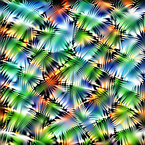
Thanks to this, we can get img with rich colour like this one
