Computing confidence intervals for predictions

Introduction

A lot of focus is made, in traditional machine learning in finding the right loss, the right regularization or the right architecture.

Once a model is trained, a lot of metrics exist to determine the value of the model.

On average, we know the performance will hold, but we don’t know much of the failure modes. We don’t know either how much the parameters would have shifted if a few data point would have moved.

These metrics seem to be as valuable as the others, so we would like to uncover the existing technics on this subject.

1 - Confidence interval for ML methods

a) Hessian based confidence interval

If you are maximising a likelihood then the covariance matrix of the estimates is (asymptotically) the inverse of the negative of the Hessian. The standard errors are the square roots of the diagonal elements of the covariance (1, 2).

This reference gives most of the required content to explain how to compute the confidence interval of the parameters of the logisitc regression.

The set of fomulas is the following :

$ \beta = \hat{\beta} +- z(0.05) SE(\beta) $

where beta is the parameter vector associated to the logistic regression, z is the function giving the z-value for a given confidence interval, SE stands for standard error of the beta.

b) The bootstrap approach

In a situation of large sample size, we can also apply a bootstrap procedure. Elements of a training set are randomly sampled with resampling.

How does this translate, following the methodology suggested in this blog post. The tedious resample approach can be replaced by a weighting using a poisson law. The approximation can be summarized as :

$ W = Poisson(1) = lim_{n=+\inf} Multinomial(n, \frac{1}{n}) $

The implementation is already super simple with a framework like sklearn. But it can be made more efficient with setting weights of the training instead of changing the data.

Pseudo code example

The priinciple is easy to illustrate. We can use the weight parameter of the fit method of sklearn model.

N_bootstrap = 100
X, Y = get_dataset()
models = list()

for _ in range(N_bootstrap):
  model = LogisticRegression()
  W = random.poisson(size=X.shape[0])
  models.append(model.fit(X, Y, W))

# Analyze models weights distribution

If this is so simple, why bother with more complicated approaches :p .

c) Quantile regression

The main idea of quantile regression is to learn a different set of models for each quantile of interval.

If you are interested in the [5, 50, 95] model, it will “just” 3 times more costly to have these estimates.

• Quantile regression works only for regression problem (at least the out of the box approach)
• It uses an asymetric loss dependent on the quantile q
• Any model can be used with this loss

Focus on the loss

The loss is defined by

where $ \rho $ is defined by :

Interpretation

Let’s take an example where q = 0.9.

At the start of the optimization, all samples have the same weights, because the x in the $\rho$ is approximately the same.

Once the weights are partially learned, the samples whose $ y - \beta X $ is superior to zero are weighted with 0.9 while the others are weighted with 0.1.

The loss will only stabilize once, the most extreme point with weight 0.9 get a smaller loss. The equilibrium is found with the majority of other data point weighted at 0.1 and with a larger loss.

d) Summary of pros and cons of methods

We can compare the methodologies presented with these tables :

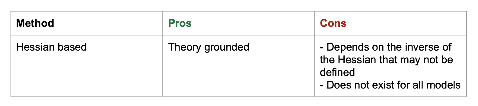
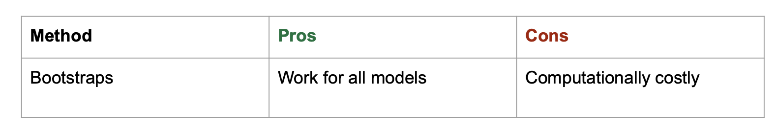
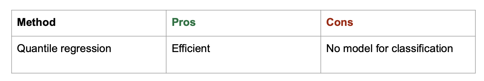
It is only a rough summary. We will see more details with examples.

2 - Comparison of methodologies on a few datasets

The presented approaches seems all trustworthy. But the actual results on data can be sometimes surprising.

So we test the different approaches on different well known datasets.

a) The affair dataset

Available on this page

It looks like the following

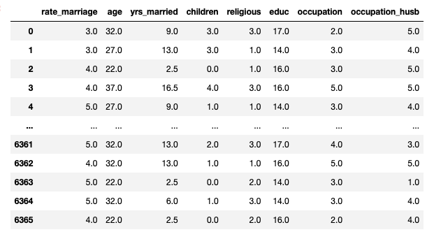
We first trained on this dataset a logistic regression using technic 1 and 2 : Hesian based and 1000 bootstraps. We compare one parameter confidence interval of the two methods on the first variable.

On this first figure, for each model, we extracted the weight corresponding to the first variable and made an histogram.

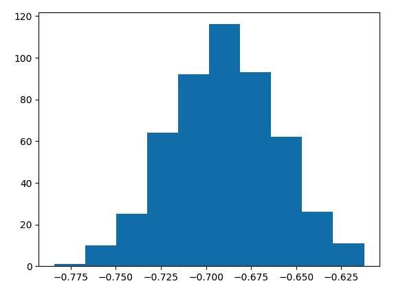
The array of the weights collected from all models allows to have a simple estimation of confidence interval by taking the nth percentile in the sorted array.

Statsmodels directly gives us the CI of a paramter when looking at the summary of the model.

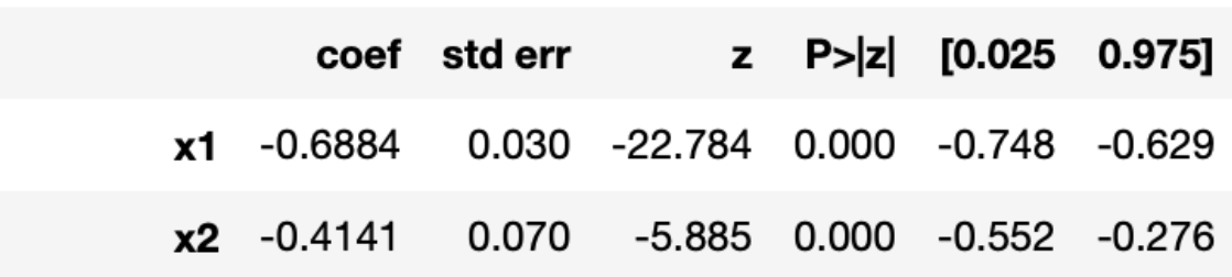
We can then compare the values found by the two methods :

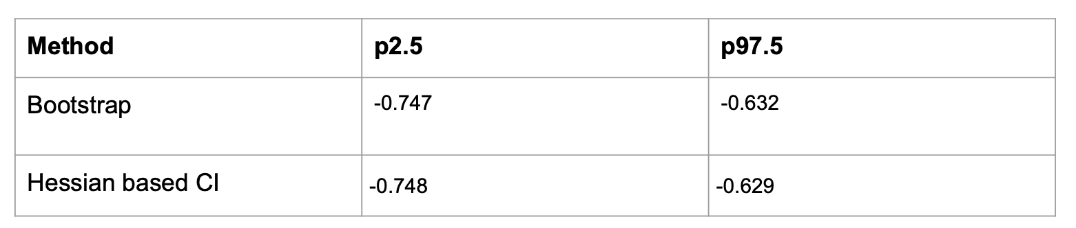
To my own surprise the two methods have approximately the same results. This is a really good results for bootstrap as one might expect less from an empirical method.

b) The Marketing modeling dataset

In this example, we work on a regression. The goal is to predict the number of item sold in each period given other variables like price or investment on marketing channels.

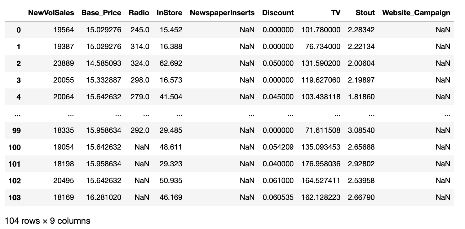
Our goal will be to determine which channel is efficient in its investment.

In this example, we will use the quantile regression method and observe what information it provides. We fit 5 models based on quantiles q=[0.05, 0.15, 0.5, 0.85, 0.95]. The modelisation will remain simple with standardization of all continuous variables and binarization of some string ones.

We get the following results, top green curve is p95, bottom blue curve is p5 and the orange middle one is the p50 :

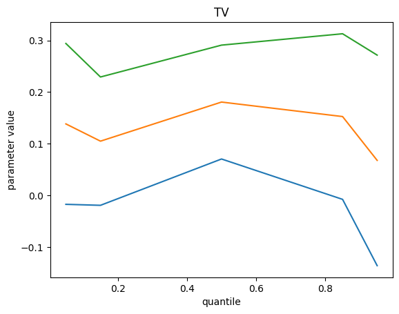
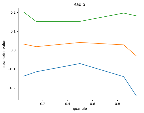
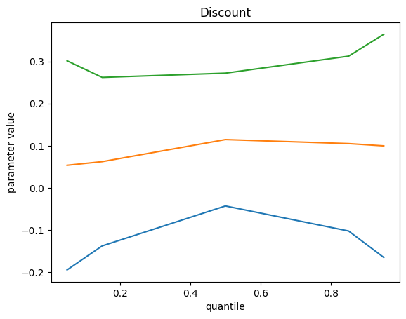
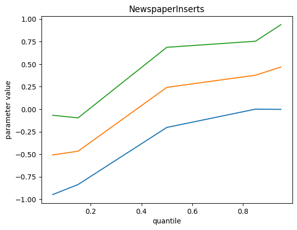
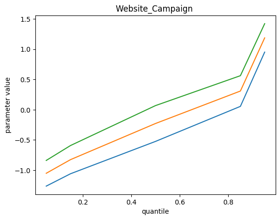
Remarks :

• Some feature importance values don’t change with quantile value
• On those which do, we can explain a different impact : investment on these channels contribute to extreme event more difficult for the model
• We do not find the bottom quantile counterpart of these extreme events. Maybe we should add something else.

We also plot the confidence interval of the final prediction

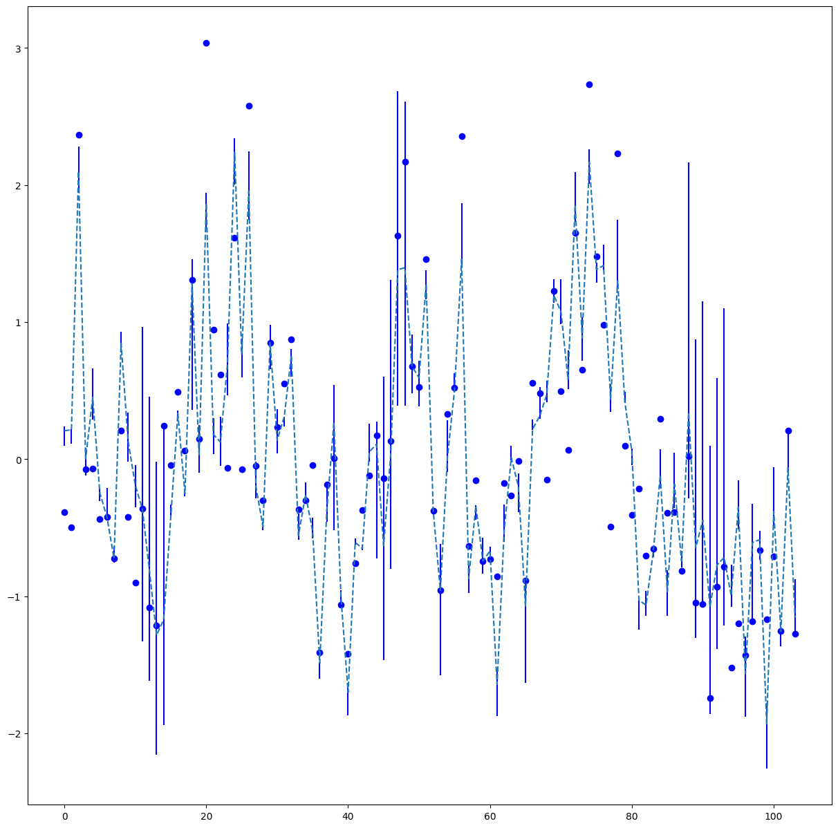
Blue points are the real data, blue line represent the confidence intervals and finally the dotted line represent the p50 fit. The target has been standardised to better see the variations.

Remarks :

• Confidence intervals don’t catch many almost zero variations
• CI sometimes get extremely large, probably because of some rare marketing events
• We seems to have more than 10% of the time a datapoint outside of the CI

Afterthoughts :

The failure to properly model some non stationary features like the stout one may explain some of the poor results.

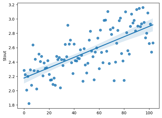
In this case, modeling the divergence from the trend could be more meaningful than standardisation over all the data. However given that we don’t understand the feature, it is difficult to assess the validity of this idea.

3 - Conclusion

• Use statsmodel, they provide really good out of box estimates
• Small dataset = you can use bootstrap, which are the most flexible
• In regression, quantile regression allows to see your results differently